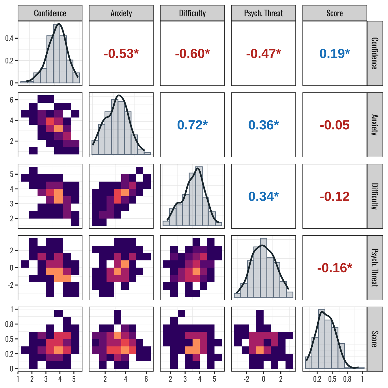
Supplementary Figure 7.1: Correlations and Variable Distributions at Baseline (Main Text, Figure 3)
7.2 Association Between Item-Level Judgments by Task
Show/Hide Code
baseline_task_compare<-data_rq1%>%filter(Timepoint=="Baseline")%>%group_by(perception)%>%nest%>%mutate( data =map(data,~group_by(.x, Participant, Part)%>%summarise(rating =mean(rating), .groups ="drop")%>%ungroup), t_test =map(data,~pairwise_t_test(.x,rating~Part, p.adjust.method ="BH", paired =TRUE)), cohens =map(data, ~cohens_d(.x, rating~Part, paired =TRUE)), tmp =map2(t_test,cohens,~full_join(.x, .y, by =join_by(.y., group1, group2, n1, n2))))%>%name_list_columns()%>%unnest(tmp)%>%select(-c(data:`.y.`))baseline_task_accuracy<-data_rq1|>filter(Timepoint=="Baseline")|>pivot_wider( names_from =perception, values_from =rating)|>summarise( .by =Part, Score =mean(Score))|>deframe()|>scales::number(accuracy =.01)# Stats to be used below:quant_d<-baseline_task_compare|>filter(group2=="Quantitative")|>ungroup()|>mutate(across(effsize, \(x)round(abs(x), 2)))|>get_summary_stats(effsize, show =c("min", "max"))compare_23<-baseline_task_compare|>filter(str_detect(group1, "Cat"), str_detect(group2, "Qual"))|>select(perception, effsize)|>deframe()|>round(2)|>abs()
Show/Hide Code
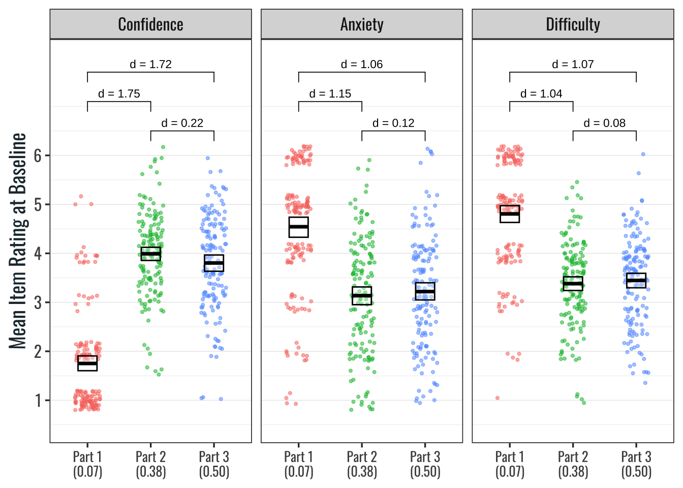
dodge_width<-.7data_rq1%>%filter(Timepoint=="Baseline")%>%group_by(Participant, Part, perception)%>%summarise(rating =mean(rating), .groups ="drop")%>%mutate( perception =factor(perception, levels =c("Confidence", "Anxiety", "Difficulty")), Part =fct_relevel(Part, "Quantitative"))%>%ggplot(aes(Part, rating, group =Part, color =Part))+geom_point( position =position_jitterdodge( jitter.width =1, jitter.height =.2, dodge.width =.7), alpha =.5, size =.8)+stat_summary( geom ="crossbar", fun.data ="mean_cl_boot", color ="black", width =.3, linewidth =.5, fill ="white", alpha =.3, position =position_dodge(dodge_width))+ggpubr::geom_bracket(aes( xmin =group1, xmax =group2, label =round(abs(effsize), 2)%>%paste("d =", .)), data =baseline_task_compare, y.position =rep(seq(6.5, 8, .6), 3), inherit.aes =FALSE, label.size =3)+facet_grid(~perception)+theme( legend.position ="none", axis.text.x =element_text( angle =0, hjust =.5, vjust =1, size =10), text =element_text(size =15))+labs(x =NULL, y ="Mean Item Rating at Baseline")+scale_y_continuous(breaks =1:6, limits =c(0.5, 8))+scale_x_discrete( labels =~paste0(paste("Part", 1:3),"\n(",baseline_task_accuracy[.x],")"))
Supplementary Figure 7.2: Mean Judgments by Physics Task Type at Baseline
Note
Supplementary Figure 7.2: Cohen’s d values for paired samples were obtained by calculating a mean perception rating for each participant by task and perception type and then dividing the mean difference by the standard deviation of the difference for each comparison. Crossbars show means and bootstrapped 95% confidence intervals. Mean accuracy for each task is shown in parentheses along the x axis.
Perception ratings were sensitive to fluctuations in performance between the physics tasks, indicating construct validity (see Supplementary Figure 7.2). For example, there was a large effect size difference in perceptions of confidence, anxiety, and difficulty between ratings on the quantitative problem solving item compared to mean ratings on both the problem categorization items and the qualitative problem solving items (Cohen’s d = 1.04 - 1.75). These differences make sense given that students performed near floor on the quantitative problem, and considerably better on the other two tasks. There was a small effect size difference between confidence ratings on the problem categorization items compared to the qualitative items (Cohen’s d = 0.22), with greater confidence reported on the problem categorization items. A likely explanation is that some of the categorization items were designed to appear simpler than they are in reality, so students may have been overconfident on those items. The difference between anxiety and difficulty ratings on the problem categorization items compared to the qualitative items was marginal (Cohen’s d = 0.12, 0.08). Overall, students’ perceptions varied with mean accuracy on the different types of items.
Source Code
# Correlations of Variables at Baseline```{r}#| label: setup#| include: falsesource("R/setup-script.R")```## Reproduction of Figure 3```{r}#| label: fig-main-fig-3#| fig-cap: Correlations and Variable Distributions at Baseline (Main Text, Figure 3)#| message: false#| warning: false#| fig-asp: 1data_rq1 %>%filter(Timepoint =="Baseline") %>%group_by(Participant, perception, Baseline_Threat) %>%summarise(rating =mean(rating), Score =mean(Score)) %>%pivot_wider(names_from = perception,values_from = rating ) %>% GGally::ggpairs(columns =c("Confidence","Anxiety","Difficulty","Baseline_Threat","Score" ),columnLabels =c("Confidence","Anxiety","Difficulty","Psych. Threat","Score" ),diag =list(continuous = fun_diag),upper =list(continuous =wrap(fun_cor_stat, method ="pearson", size =6)),lower =list(continuous = fun_lower) ) +theme(panel.spacing =unit(3, "mm"), axis.text =element_text(size =9)) +scale_x_continuous(labels =~round(., 1)) +scale_y_continuous(labels =~round(., 1))```## Association Between Item-Level Judgments by Task```{r}#| label: baseline-task-comparebaseline_task_compare <- data_rq1 %>%filter(Timepoint =="Baseline") %>%group_by(perception) %>% nest %>%mutate(data =map( data,~group_by(.x, Participant, Part) %>%summarise(rating =mean(rating), .groups ="drop") %>% ungroup ),t_test =map( data,~pairwise_t_test( .x, rating ~ Part,p.adjust.method ="BH",paired =TRUE ) ),cohens =map(data, ~cohens_d(.x, rating ~ Part, paired =TRUE)),tmp =map2( t_test, cohens,~full_join(.x, .y, by =join_by(.y., group1, group2, n1, n2)) ) ) %>%name_list_columns() %>%unnest(tmp) %>%select(-c(data:`.y.`))baseline_task_accuracy <- data_rq1 |>filter(Timepoint =="Baseline") |>pivot_wider(names_from = perception,values_from = rating ) |>summarise(.by = Part,Score =mean(Score) ) |>deframe() |> scales::number(accuracy = .01)# Stats to be used below:quant_d <- baseline_task_compare |>filter(group2 =="Quantitative") |>ungroup() |>mutate(across(effsize, \(x) round(abs(x), 2))) |>get_summary_stats(effsize, show =c("min", "max"))compare_23 <- baseline_task_compare |>filter(str_detect(group1, "Cat"), str_detect(group2, "Qual")) |>select(perception, effsize) |>deframe() |>round(2) |>abs()``````{r}#| label: fig-judgment-by-task#| fig-cap: Mean Judgments by Physics Task Type at Baselinedodge_width <- .7data_rq1 %>%filter(Timepoint =="Baseline") %>%group_by(Participant, Part, perception) %>%summarise(rating =mean(rating), .groups ="drop") %>%mutate(perception =factor( perception,levels =c("Confidence", "Anxiety", "Difficulty") ),Part =fct_relevel(Part, "Quantitative") ) %>%ggplot(aes(Part, rating, group = Part, color = Part)) +geom_point(position =position_jitterdodge(jitter.width =1,jitter.height = .2,dodge.width = .7 ),alpha = .5,size = .8 ) +stat_summary(geom ="crossbar",fun.data ="mean_cl_boot",color ="black",width = .3,linewidth = .5,fill ="white",alpha = .3,position =position_dodge(dodge_width) ) + ggpubr::geom_bracket(aes(xmin = group1,xmax = group2,label =round(abs(effsize), 2) %>%paste("d =", .) ),data = baseline_task_compare,y.position =rep(seq(6.5, 8, .6), 3),inherit.aes =FALSE,label.size =3 ) +facet_grid(~perception) +theme(legend.position ="none",axis.text.x =element_text(angle =0,hjust = .5,vjust =1,size =10 ),text =element_text(size =15) ) +labs(x =NULL, y ="Mean Item Rating at Baseline") +scale_y_continuous(breaks =1:6, limits =c(0.5, 8)) +scale_x_discrete(labels =~paste0(paste("Part", 1:3),"\n(", baseline_task_accuracy[.x],")" ) )```:::{.callout-note}@fig-judgment-by-task: Cohen’s *d* values for paired samples were obtained by calculating a mean perception rating for each participant by task and perception type and then dividing the mean difference by the standard deviation of the difference for each comparison. Crossbars show means and bootstrapped 95% confidence intervals. Mean accuracy for each task is shown in parentheses along the *x* axis.:::Perception ratings were sensitive to fluctuations in performance between the physics tasks, indicating construct validity (see @fig-judgment-by-task). For example, there was a large effect size difference in perceptions of confidence, anxiety, and difficulty between ratings on the quantitative problem solving item compared to mean ratings on both the problem categorization items and the qualitative problem solving items (Cohen’s *d* = `{r} quant_d$min` - `{r} quant_d$max`). These differences make sense given that students performed near floor on the quantitative problem, and considerably better on the other two tasks. There was a small effect size difference between confidence ratings on the problem categorization items compared to the qualitative items (Cohen’s *d* = `{r} compare_23["Confidence"]`), with greater confidence reported on the problem categorization items. A likely explanation is that some of the categorization items were designed to appear simpler than they are in reality, so students may have been overconfident on those items. The difference between anxiety and difficulty ratings on the problem categorization items compared to the qualitative items was marginal (Cohen’s *d* = `{r} compare_23["Anxiety"]`, `{r} compare_23["Difficulty"]`). Overall, students’ perceptions varied with mean accuracy on the different types of items.